Car Price¶

[1]:

import numpy as np
import pandas as pd
import matplotlib.pyplot as plt
import seaborn as sns

[2]:

df_test= pd.read_csv("test_car_details.csv")
df_train = pd.read_csv("train_car_details.csv")

[3]:

print(df_train.columns)
print(df_test.columns)

Index(['Id', 'name', 'year', 'selling_price', 'km_driven', 'fuel',
       'seller_type', 'transmission', 'owner', 'mileage', 'engine',
       'max_power', 'torque', 'seats'],
      dtype='object')
Index(['Id', 'name', 'year', 'km_driven', 'fuel', 'seller_type',
       'transmission', 'owner', 'mileage', 'engine', 'max_power', 'torque',
       'seats'],
      dtype='object')

Objetivo¶

Um dos problemas que ocorrem na OLX da Índia, pela baixa volumetria de dados, é a empresa não conseguir estimar um preço de venda para o carro do seu cliente baseado em algumas características do veículo. O objetivo é estimar tal valor a partir de dados do concorrente (CarDekho).

Análise qualitativa e quantitativa dos dados¶

[4]:

#Verificando as variáveis
df_train.head()

[4]:

	Id	name	year	selling_price	km_driven	fuel	seller_type	transmission	owner	mileage	engine	max_power	torque	seats
0	1	Hyundai Santro GLS I - Euro I	1999	80000	110000	Petrol	Individual	Manual	Second Owner	NaN	NaN	NaN	NaN	NaN
1	2	Maruti Ertiga VDI	2012	459999	87000	Diesel	Individual	Manual	First Owner	20.77 kmpl	1248 CC	88.76 bhp	200Nm@ 1750rpm	7.0
2	3	BMW 3 Series 320d Luxury Line	2010	1100000	102000	Diesel	Dealer	Automatic	First Owner	19.62 kmpl	1995 CC	187.74 bhp	400Nm@ 1750-2500rpm	5.0
3	4	Tata New Safari DICOR 2.2 EX 4x2	2009	229999	212000	Diesel	Individual	Manual	Third Owner	11.57 kmpl	2179 CC	138.1 bhp	320Nm@ 1700-2700rpm	7.0
4	5	Toyota Fortuner 3.0 Diesel	2010	800000	125000	Diesel	Individual	Manual	Second Owner	11.5 kmpl	2982 CC	171 bhp	343Nm@ 1400-3400rpm	7.0

[5]:

df_train = df_train.iloc[:,1:] #retirando a coluna de id

Id = df_test.Id
df_test = df_test.iloc[:,1:] #retirando a coluna de id

Analise de dados nulos¶

[6]:

#Verificado a quantidade de NaN por atributo
df_train.isna().sum()

[6]:

name               0
year               0
selling_price      0
km_driven          0
fuel               0
seller_type        0
transmission       0
owner              0
mileage          157
engine           157
max_power        151
torque           158
seats            157
dtype: int64

[7]:

#Porcentagem de nan por atributo
print(100*df_train.isna().sum()/len(df_train))

name             0.000000
year             0.000000
selling_price    0.000000
km_driven        0.000000
fuel             0.000000
seller_type      0.000000
transmission     0.000000
owner            0.000000
mileage          2.759712
engine           2.759712
max_power        2.654245
torque           2.777290
seats            2.759712
dtype: float64

[8]:

#Porcentagem de nan por atributo no test
print(100*df_test.isna().sum()/len(df_test))

name            0.0
year            0.0
km_driven       0.0
fuel            0.0
seller_type     0.0
transmission    0.0
owner           0.0
mileage         0.0
engine          0.0
max_power       0.0
torque          0.0
seats           0.0
dtype: float64

Pelo fatos dos NaN’s estar majoritariamente presente nas mesmas linhas e por representar um baixo volume em relação ao total (menos de 3%), tais linhas serão retiradas.

[9]:

print(f'Quantidade de linhas totais: ', df_train.shape[0])
# Remove as linhas com NaN
df_train = df_train.dropna(axis=0)
print(f'Quantidade de linhas após retirada dos NaNs: ', df_train.shape[0])
#Aproximadamente 3% de linhas eliminadas

Quantidade de linhas totais:  5689
Quantidade de linhas após retirada dos NaNs:  5531

Categoria das variaveis¶

Os dados são compostos pelas variáveis:

Variaveis quantitativas discreta:
Ano de fabricacao do carro (year)
Qtd de Km dirigidos (km_driven)
Potência máxima do motor (max_power)
Qtd de acentos (seats)
Variaveis quantitativas continuas:
Quilometragem por litro (mileage)
Potencia do motor (engine)
Preço de venda (selling_price) Valor a ser predito
Variaveis qualitativas nominais:
nome do carro (name)
tipo de combustivel utilizado (fuel)
tipo de vendendor (seller_type)
transmissao (transmission)
Torque: responsável pela capacidade do motor produzir força motriz, ou seja, o movimento giratório
Variaveis qualitativas ordinais:
Quantos donos ja possuiram o carro (owner)

Nota-se que 4 variáveis são numéricas, mas é necessário uma tratativa para retirar as strings que representam a unidade de medida. Ao todo, considerando as variáveis que precisam ser tratadas, há 7 variáveis numéricas e 6 variáveis categóricas qualitativas.

Retirando a palavra owner da coluna owner, retirando a unidade de medida de mileage, engine e max power e retirando a segunda unidade de medida utilizada no torque (rpm) e deixando apenas a unidade Nm¶

[10]:

df1 = df_train.copy()

[11]:

colunas = ['owner', 'mileage', 'engine',
       'max_power', 'torque']

[12]:

#base de treino
for i in colunas:
  df1[i] = df1[i].str.split(' ').str[0]

#Na base de test
for i in colunas:
  df_test[i] = df_test[i].str.split(' ').str[0]

Retirando a unidade de medida do torque¶

[13]:

#Retirando a unidade de medida do torque
df1['torque'] = df1['torque'].str.replace('Nm@', '', regex=True).replace('nm@', '', regex=True).replace('@', '', regex=True).replace('Nm', '', regex=True).replace('NM', '', regex=True).replace('kgm', '', regex=True)

#no test
df_test['torque'] = df_test['torque'].str.replace('Nm@', '', regex=True).replace('nm@', '', regex=True).replace('@', '', regex=True).replace('Nm', '', regex=True).replace('NM', '', regex=True).replace('kgm', '', regex=True)

[14]:

df1[df1['torque'] == '110(11.2)']

[14]:

	name	year	selling_price	km_driven	fuel	seller_type	transmission	owner	mileage	engine	max_power	torque	seats
1954	Honda Jazz Select Edition Active	2011	350000	80000	Petrol	Individual	Manual	Second	16.0	1198	90	110(11.2)	5.0

Nao temos esse problema na base de teste

Tratando a linha com torque (11.2) no treino¶

[15]:

#eliminando a linha com toque = 110(11.2)
df1.drop(df1.loc[df1['torque'] == '110(11.2)'].index, inplace=True)

Tratando linha 380(38.7) no torque (base teste)¶

[16]:

df_test[df_test['torque'] == '380(38.7)']

[16]:

	name	year	km_driven	fuel	seller_type	transmission	owner	mileage	engine	max_power	torque	seats
885	Ford Endeavour Hurricane Limited Edition	2013	110000	Diesel	Individual	Automatic	Third	12.8	2953	156	380(38.7)	7.0

Nao podemos eliminar linhas da base de teste

[17]:

df_test[df_test['torque'] == '380(38.7)']

[17]:

	name	year	km_driven	fuel	seller_type	transmission	owner	mileage	engine	max_power	torque	seats
885	Ford Endeavour Hurricane Limited Edition	2013	110000	Diesel	Individual	Automatic	Third	12.8	2953	156	380(38.7)	7.0

[18]:

df_test.torque.replace('380(38.7)', '380', inplace= True)

[19]:

df_test[df_test['torque'] == '380(38.7)']

[19]:

	name	year	km_driven	fuel	seller_type	transmission	owner	mileage	engine	max_power	torque	seats

Analisando nome dos carros¶

[20]:

#Colocando a marca e modelo do carro em um dicionario juntamente com sua frequência no conjunto
import collections
agrupamento = df1['name']
counter=collections.Counter(agrupamento)

[21]:

#Colocando a frequencia em uma lista para poder contar a qtd de itens diferentes
contador = []
for i in sorted(counter, key = counter.get, reverse = True):
    contador.append(counter[i])
print("Quantidade de modelos de carros distintos: ",len(contador))
print("A maior quantidade de um único modelo de carro: ",max(contador))

Quantidade de modelos de carros distintos:  1706
A maior quantidade de um único modelo de carro:  92

Como o nome dos carros é muito variado, não é interessante estar presente no modelo, porém, a informação da marca do carro pode ser importante, assim como outras informações oriundas da própria base.

Feature engineering¶

Criando a feature marca¶

[22]:

#Criando a coluna marca
df1['brand'] = df1['name'].str.split(' ').str[0]

#para a base de teste
df_test['brand'] = df_test['name'].str.split(' ').str[0]

[23]:

df1['brand'].unique()

[23]:

array(['Maruti', 'BMW', 'Tata', 'Toyota', 'Hyundai', 'Chevrolet', 'Honda',
       'Jaguar', 'Renault', 'Mahindra', 'Volkswagen', 'Ford', 'Skoda',
       'Datsun', 'Fiat', 'Volvo', 'Nissan', 'Mercedes-Benz', 'Kia',
       'Jeep', 'Audi', 'Isuzu', 'Lexus', 'Land', 'Force', 'Mitsubishi',
       'Ambassador', 'Daewoo', 'MG', 'Ashok'], dtype=object)

[24]:

df_test['brand'].unique()

[24]:

array(['Tata', 'Maruti', 'Mahindra', 'Hyundai', 'Volvo', 'Jaguar',
       'Chevrolet', 'Jeep', 'Honda', 'Toyota', 'Kia', 'Ford', 'Lexus',
       'Skoda', 'BMW', 'Fiat', 'Renault', 'Nissan', 'Datsun',
       'Mercedes-Benz', 'Volkswagen', 'Opel', 'Mitsubishi', 'Ambassador',
       'Audi', 'Land', 'Isuzu', 'Force'], dtype=object)

Criando a coluna idade do carro¶

[25]:

#Criando a coluna idade do carro
df1['age'] = 2021 - df1.year

#para a base de teste
df_test['age'] = 2021 - df_test.year

Retirando a coluna name e year¶

[26]:

del df1["name"] #retirando a coluna name
del df1["year"] #retirando a coluna year
del df1["torque"] #retirando a coluna year ## 0.9705529686331869 (sem torque) gradiente
#del df1["seats"] #retirando a coluna year ## 0.9719490890165687 (sem seats e torque) gradiente
#del df1["engine"] #retirando a coluna year ### 0.9723490022839645 (sem engine, seats e torque) gradiente


del df_test["name"] #retirando a coluna name
del df_test["year"] #retirando a coluna year
del df_test["torque"] #retirando a coluna torque
#del df_test["seats"] #retirando a coluna year
#del df_test["engine"] #retirando a coluna year

Adequando o tipo de dado de algumas variáveis¶

[27]:

#Mudando o tipo de dado de algumas variáveis
df1['mileage'] = pd.to_numeric(df1['mileage'])
df1['max_power'] = pd.to_numeric(df1['max_power'])
df1['engine'] = pd.to_numeric(df1['engine'])
df1['seats'] = pd.to_numeric(df1['seats'])
#df1['torque'] = pd.to_numeric(df1['torque'])

#Base de Teste
df_test['mileage'] = pd.to_numeric(df_test['mileage'])
df_test['max_power'] = pd.to_numeric(df_test['max_power'])
df_test['engine'] = pd.to_numeric(df_test['engine'])
df_test['seats'] = pd.to_numeric(df_test['seats'])
#df_test['torque'] = pd.to_numeric(df_test['torque'])

Transformar as variaveis categoricas para a regressão¶

Substituicao variaveis categoricas por rótulos numéricos¶

[28]:

from sklearn import preprocessing
le = preprocessing.LabelEncoder()
#base de treino
for i in range(0, len(df1.columns.values)):
  if df1.dtypes[i] == 'O':
    df1.iloc[:, i] = le.fit_transform(df1.iloc[:, i]).astype('str')

#Na base de test
for i in range(0, len(df_test.columns.values)):
  if df_test.dtypes[i] == 'O':
    df_test.iloc[:, i] = le.fit_transform(df_test.iloc[:, i]).astype('str')

[29]:

df1.info()

<class 'pandas.core.frame.DataFrame'>
Int64Index: 5530 entries, 1 to 5688
Data columns (total 12 columns):
 #   Column         Non-Null Count  Dtype
---  ------         --------------  -----
 0   selling_price  5530 non-null   int64
 1   km_driven      5530 non-null   int64
 2   fuel           5530 non-null   object
 3   seller_type    5530 non-null   object
 4   transmission   5530 non-null   object
 5   owner          5530 non-null   object
 6   mileage        5530 non-null   float64
 7   engine         5530 non-null   int64
 8   max_power      5530 non-null   float64
 9   seats          5530 non-null   float64
 10  brand          5530 non-null   object
 11  age            5530 non-null   int64
dtypes: float64(3), int64(4), object(5)
memory usage: 561.6+ KB

[30]:

df1.head(5)

[30]:

	selling_price	km_driven	fuel	seller_type	transmission	owner	mileage	engine	max_power	seats	brand	age
1	459999	87000	1	1	1	0	20.77	1248	88.76	7.0	20	9
2	1100000	102000	1	0	0	0	19.62	1995	187.74	5.0	3	11
3	229999	212000	1	1	1	4	11.57	2179	138.10	7.0	26	12
4	800000	125000	1	1	1	2	11.50	2982	171.00	7.0	27	11
5	180000	25000	3	1	1	2	19.70	796	46.30	5.0	20	11

Temos agora todas as variaveis numericas para utilizar na nossa regressao

[33]:

plt.figure(figsize=(16, 6))
# define the mask to set the values in the upper triangle to True
mask = np.triu(np.ones_like(df1.corr(), dtype=bool))
heatmap = sns.heatmap(df1.corr(), mask=mask, vmin=-1, vmax=1, annot=True, cmap='BrBG')
heatmap.set_title('Correlation Heatmap', fontdict={'fontsize':18}, pad=16);

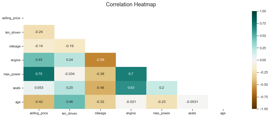
../../_images/Jupyter_Car_Price_Car_Price_55_0.png

Correlacoes muito altas entre variaveis do treino poderiam ser reduntantes, observamos que isso nao ocorre

Analise das variaveis quantitativas¶

[34]:

c = ['selling_price','km_driven','mileage','engine', 'max_power', 'seats', 'age']

for i in c:

  sns.set(style="ticks")

  x = df1[i]
  coluna = i
  mu = round(x.mean(),2) # mean of distribution
  sigma = round(x.std(),2)  # standard deviation of distribution

  f, (ax_box, ax_hist) = plt.subplots(2)

  sns.boxplot(x=x, ax=ax_box)
  sns.histplot(x=x, ax=ax_hist)

  ax_box.set(yticks=[])
  sns.despine(ax=ax_hist)
  sns.despine(ax=ax_box, left=True)
  ax_box.set_title('Boxplot e Histograma de {}\n $\mu={}$, $\sigma={}$'.format(coluna, mu,sigma))

plt.show()

../../_images/Jupyter_Car_Price_Car_Price_58_0.png

../../_images/Jupyter_Car_Price_Car_Price_58_1.png

../../_images/Jupyter_Car_Price_Car_Price_58_2.png

../../_images/Jupyter_Car_Price_Car_Price_58_3.png

../../_images/Jupyter_Car_Price_Car_Price_58_4.png

../../_images/Jupyter_Car_Price_Car_Price_58_5.png

../../_images/Jupyter_Car_Price_Car_Price_58_6.png

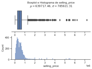
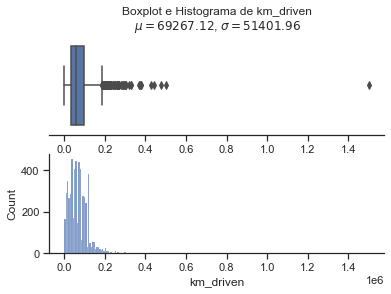
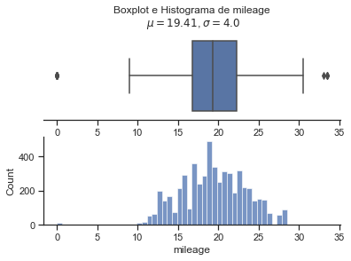
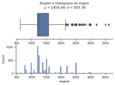
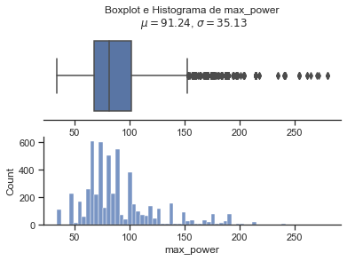
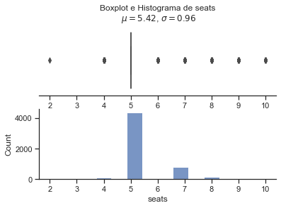
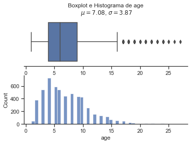
Nota se que a variavel que devemos prever, selling price tem uma altissima variancia e quase todas as variaveis quantitativas possuem outliers

Preparacao dos dados¶

antes de fazer a feature selection vamos normalizar e separar o que deve ser predito das variaveis duvida: deve ser normalizado antes da feature selection?

[35]:

df1.head()

[35]:

	selling_price	km_driven	fuel	seller_type	transmission	owner	mileage	engine	max_power	seats	brand	age
1	459999	87000	1	1	1	0	20.77	1248	88.76	7.0	20	9
2	1100000	102000	1	0	0	0	19.62	1995	187.74	5.0	3	11
3	229999	212000	1	1	1	4	11.57	2179	138.10	7.0	26	12
4	800000	125000	1	1	1	2	11.50	2982	171.00	7.0	27	11
5	180000	25000	3	1	1	2	19.70	796	46.30	5.0	20	11

[36]:

colunas = df1.iloc[:,1:].columns

[37]:

colunas

[37]:

Index(['km_driven', 'fuel', 'seller_type', 'transmission', 'owner', 'mileage',
       'engine', 'max_power', 'seats', 'brand', 'age'],
      dtype='object')

Padronizacao¶

Vamos padronizar a base a ser predita tbm

Transformar para formato numpy para nao termos erro na normalizacao

[59]:

data = df1.to_numpy()
nrow,ncol = df1.shape
y = data[:,:1]
X = data[:,1:]

[39]:

from sklearn.preprocessing import StandardScaler
from sklearn.preprocessing import MinMaxScaler

scaler_train = StandardScaler()
#scaler_train = MinMaxScaler()
X = scaler_train.fit_transform(X)

#Padronizando os precos tbm
#scaler_train = StandardScaler()
#scaler_train = MinMaxScaler()
#y = scaler_train.fit_transform(y)

#Vamos padronizar o teste tbm
scaler_train = StandardScaler()
#scaler_train = MinMaxScaler()
df_test1 = scaler_train.fit_transform(df_test)

[40]:

print(y.shape)
print(X.shape)

(5530, 1)
(5530, 11)

Separacao treino e teste¶

[41]:

from sklearn.model_selection import train_test_split

X_train, X_test, y_train, y_test = train_test_split(X, y, test_size = 0.2, random_state = 4)

Catboost¶

[43]:

from catboost import CatBoostRegressor
from sklearn.model_selection import GridSearchCV

[44]:

 parameters = {'depth'         : [6,8,10],
                  'learning_rate' : [0.01, 0.05, 0.1],
                  'iterations'    : [30, 50, 100]
                 }
model_CBR = CatBoostRegressor(logging_level='Silent')

eval_set=[(X_train, y_train), (X_test, y_test)]

[45]:

%%time

grid = GridSearchCV(estimator=model_CBR, param_grid = parameters, cv = 10, n_jobs=-1, scoring='r2')
grid.fit(X_train, y_train, eval_set=eval_set, early_stopping_rounds=10)
#grid.fit(X_train, y_train)



print("Melhor modelo: {}".format(grid.best_estimator_))
print("Melhor score: {}".format(grid.best_score_))

Melhor modelo: <catboost.core.CatBoostRegressor object at 0x0000021C7A608F10>
Melhor score: 0.9636405747742944
Wall time: 4min

[46]:

from sklearn.metrics import r2_score
y_predict = grid.predict(X_test)

#rmse = np.sqrt(mean_squared_error(y_test,y_linear_pred))
r2 = r2_score(y_test,y_predict)
print(r2)

0.9525834925856915

Feature Selection¶

https://www.analyseup.com/learn-python-for-data-science/python-random-forest-feature-importance-plot.html

[47]:

def plot_feature_importance(importance,names,model_type):

    #Create arrays from feature importance and feature names
    feature_importance = np.array(importance)
    feature_names = np.array(names)

    #Create a DataFrame using a Dictionary
    data={'feature_names':feature_names,'feature_importance':feature_importance}
    fi_df = pd.DataFrame(data)

    #Sort the DataFrame in order decreasing feature importance
    fi_df.sort_values(by=['feature_importance'], ascending=False,inplace=True)

    #Define size of bar plot
    plt.figure(figsize=(10,8))
    #Plot Searborn bar chart
    sns.barplot(x=fi_df['feature_importance'], y=fi_df['feature_names'])
    #Add chart labels
    plt.title(model_type + 'FEATURE IMPORTANCE')
    plt.xlabel('FEATURE IMPORTANCE')
    plt.ylabel('FEATURE NAMES')

[48]:

plot_feature_importance(grid.best_estimator_.get_feature_importance(),colunas,'CATBOOST ')

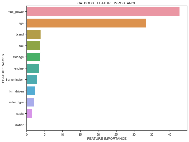
../../_images/Jupyter_Car_Price_Car_Price_81_0.png

Vamos tirar as colunas com menos importancia¶

[49]:

df1.head()
c = ['owner', 'seats', 'seller_type']
df2 = df1.drop(labels = c, axis = 1)

df_test2 = df_test.drop(labels = c, axis = 1)

[50]:

df2

[50]:

	selling_price	km_driven	fuel	transmission	mileage	engine	max_power	brand	age
1	459999	87000	1	1	20.77	1248	88.76	20	9
2	1100000	102000	1	0	19.62	1995	187.74	3	11
3	229999	212000	1	1	11.57	2179	138.10	26	12
4	800000	125000	1	1	11.50	2982	171.00	27	11
5	180000	25000	3	1	19.70	796	46.30	20	11
...	...	...	...	...	...	...	...	...	...
5684	550000	20000	3	1	18.90	1197	82.00	11	4
5685	360000	81000	1	1	19.01	1461	108.45	24	8
5686	310000	70000	1	1	19.30	1248	73.90	20	10
5687	650000	57000	1	1	23.65	1248	88.50	20	6
5688	420000	90000	1	1	24.40	1120	71.01	11	7

5530 rows × 9 columns

[51]:

from sklearn.preprocessing import StandardScaler
from sklearn.preprocessing import MinMaxScaler

data = df2.to_numpy()
nrow,ncol = df2.shape
y = data[:,:1]
X = data[:,1:]

scaler_train = StandardScaler()
#scaler_train = MinMaxScaler()
X = scaler_train.fit_transform(X)

#Vamos padronizar o teste tbm
scaler_train = StandardScaler()
#scaler_train = MinMaxScaler()
df_test2 = scaler_train.fit_transform(df_test2)

[52]:

from sklearn.model_selection import train_test_split

X_train, X_test, y_train, y_test = train_test_split(X, y, test_size = 0.2, random_state = 4)

[53]:

parameters = {'depth'         : [6,8,10],
                  'learning_rate' : [0.01, 0.05, 0.1],
                  'iterations'    : [30, 50, 100]
                 }
model_CBR = CatBoostRegressor()

eval_set=[(X_train, y_train), (X_test, y_test)]

[54]:

%%time

grid = GridSearchCV(estimator=model_CBR, param_grid = parameters, cv = 10, n_jobs=-1, scoring='r2')
grid.fit(X_train, y_train, eval_set=eval_set, early_stopping_rounds=10)
#grid.fit(X_train, y_train)

y_predict = grid.predict(X_test)

#rmse = np.sqrt(mean_squared_error(y_test,y_linear_pred))
#r2 = r2_score(y_test,y_linear_pred)

print("Melhor modelo: {}".format(grid.best_estimator_))
print("Melhor score: {}".format(grid.best_score_))

0:      learn: 725099.3360888   test: 725099.3360888    test1: 725838.2268251   best: 725838.2268251 (0)        total: 41.3ms   remaining: 4.09s
1:      learn: 667962.7502607   test: 667962.7502607    test1: 670005.4649577   best: 670005.4649577 (1)        total: 47.4ms   remaining: 2.32s
2:      learn: 618026.2240742   test: 618026.2240742    test1: 621886.9502452   best: 621886.9502452 (2)        total: 54.6ms   remaining: 1.76s
3:      learn: 570637.0627416   test: 570637.0627416    test1: 578186.2612178   best: 578186.2612178 (3)        total: 60.7ms   remaining: 1.46s
4:      learn: 527755.3300552   test: 527755.3300552    test1: 536947.9038419   best: 536947.9038419 (4)        total: 67.1ms   remaining: 1.27s
5:      learn: 490277.1990580   test: 490277.1990580    test1: 502595.3096877   best: 502595.3096877 (5)        total: 73.5ms   remaining: 1.15s
6:      learn: 453374.2521619   test: 453374.2521619    test1: 467777.7143207   best: 467777.7143207 (6)        total: 80.3ms   remaining: 1.07s
7:      learn: 420792.5779912   test: 420792.5779912    test1: 437861.6946392   best: 437861.6946392 (7)        total: 90.2ms   remaining: 1.04s
8:      learn: 393043.0440251   test: 393043.0440251    test1: 411090.6830783   best: 411090.6830783 (8)        total: 97.3ms   remaining: 984ms
9:      learn: 367221.8236830   test: 367221.8236830    test1: 386919.3392056   best: 386919.3392056 (9)        total: 107ms    remaining: 966ms
10:     learn: 343181.0694443   test: 343181.0694443    test1: 364792.0635716   best: 364792.0635716 (10)       total: 118ms    remaining: 957ms
11:     learn: 322896.6381826   test: 322896.6381826    test1: 345040.7307973   best: 345040.7307973 (11)       total: 125ms    remaining: 916ms
12:     learn: 302845.9618204   test: 302845.9618204    test1: 326860.5565415   best: 326860.5565415 (12)       total: 135ms    remaining: 902ms
13:     learn: 286641.4715800   test: 286641.4715800    test1: 312219.6312316   best: 312219.6312316 (13)       total: 143ms    remaining: 879ms
14:     learn: 270952.0744893   test: 270952.0744893    test1: 297170.7323797   best: 297170.7323797 (14)       total: 153ms    remaining: 869ms
15:     learn: 258475.3925918   test: 258475.3925918    test1: 286340.8212579   best: 286340.8212579 (15)       total: 164ms    remaining: 863ms
16:     learn: 246371.0312132   test: 246371.0312132    test1: 275079.9896599   best: 275079.9896599 (16)       total: 172ms    remaining: 840ms
17:     learn: 233887.0889817   test: 233887.0889817    test1: 264771.1551038   best: 264771.1551038 (17)       total: 183ms    remaining: 832ms
18:     learn: 222216.5469460   test: 222216.5469460    test1: 255136.6229553   best: 255136.6229553 (18)       total: 189ms    remaining: 807ms
19:     learn: 212494.4651008   test: 212494.4651008    test1: 246835.1105830   best: 246835.1105830 (19)       total: 198ms    remaining: 793ms
20:     learn: 204382.3914991   test: 204382.3914991    test1: 240594.7171910   best: 240594.7171910 (20)       total: 206ms    remaining: 775ms
21:     learn: 197076.2687288   test: 197076.2687288    test1: 234047.3517937   best: 234047.3517937 (21)       total: 214ms    remaining: 759ms
22:     learn: 190717.9316182   test: 190717.9316182    test1: 229118.7773587   best: 229118.7773587 (22)       total: 224ms    remaining: 750ms
23:     learn: 184265.7333922   test: 184265.7333922    test1: 224184.7455733   best: 224184.7455733 (23)       total: 233ms    remaining: 738ms
24:     learn: 179223.7916875   test: 179223.7916875    test1: 219812.4763748   best: 219812.4763748 (24)       total: 240ms    remaining: 719ms
25:     learn: 174527.9822117   test: 174527.9822117    test1: 214888.9196695   best: 214888.9196695 (25)       total: 247ms    remaining: 704ms
26:     learn: 170404.2989815   test: 170404.2989815    test1: 211053.6780763   best: 211053.6780763 (26)       total: 254ms    remaining: 687ms
27:     learn: 166863.7350093   test: 166863.7350093    test1: 208784.3367464   best: 208784.3367464 (27)       total: 261ms    remaining: 672ms
28:     learn: 163260.1751759   test: 163260.1751759    test1: 205808.8396433   best: 205808.8396433 (28)       total: 270ms    remaining: 661ms
29:     learn: 158926.3923587   test: 158926.3923587    test1: 202478.9809685   best: 202478.9809685 (29)       total: 277ms    remaining: 647ms
30:     learn: 155785.3469715   test: 155785.3469715    test1: 200400.2700177   best: 200400.2700177 (30)       total: 285ms    remaining: 635ms
31:     learn: 152749.5027848   test: 152749.5027848    test1: 198254.6641147   best: 198254.6641147 (31)       total: 293ms    remaining: 623ms
32:     learn: 150483.6658493   test: 150483.6658493    test1: 196047.9345613   best: 196047.9345613 (32)       total: 300ms    remaining: 609ms
33:     learn: 148229.8724341   test: 148229.8724341    test1: 194514.8600443   best: 194514.8600443 (33)       total: 308ms    remaining: 597ms
34:     learn: 146027.7013355   test: 146027.7013355    test1: 192266.2622987   best: 192266.2622987 (34)       total: 314ms    remaining: 584ms
35:     learn: 144245.4701191   test: 144245.4701191    test1: 191552.0168309   best: 191552.0168309 (35)       total: 322ms    remaining: 572ms
36:     learn: 142413.2536117   test: 142413.2536117    test1: 190117.7821396   best: 190117.7821396 (36)       total: 331ms    remaining: 563ms
37:     learn: 140688.3204281   test: 140688.3204281    test1: 188455.4328949   best: 188455.4328949 (37)       total: 340ms    remaining: 554ms
38:     learn: 139066.2852420   test: 139066.2852420    test1: 187131.2301431   best: 187131.2301431 (38)       total: 346ms    remaining: 541ms
39:     learn: 137603.2707736   test: 137603.2707736    test1: 185678.7582810   best: 185678.7582810 (39)       total: 353ms    remaining: 529ms
40:     learn: 136068.0198434   test: 136068.0198434    test1: 184205.7321537   best: 184205.7321537 (40)       total: 362ms    remaining: 521ms
41:     learn: 134378.2331538   test: 134378.2331538    test1: 183290.2839965   best: 183290.2839965 (41)       total: 371ms    remaining: 512ms
42:     learn: 132782.4541325   test: 132782.4541325    test1: 182169.0617821   best: 182169.0617821 (42)       total: 378ms    remaining: 501ms
43:     learn: 131790.3338328   test: 131790.3338328    test1: 181371.1566799   best: 181371.1566799 (43)       total: 386ms    remaining: 492ms
44:     learn: 130880.2599549   test: 130880.2599549    test1: 180683.8795768   best: 180683.8795768 (44)       total: 393ms    remaining: 480ms
45:     learn: 129808.2123748   test: 129808.2123748    test1: 180036.1907090   best: 180036.1907090 (45)       total: 399ms    remaining: 468ms
46:     learn: 129303.5785381   test: 129303.5785381    test1: 179738.2600447   best: 179738.2600447 (46)       total: 407ms    remaining: 459ms
47:     learn: 128048.3689670   test: 128048.3689670    test1: 178556.9712466   best: 178556.9712466 (47)       total: 415ms    remaining: 449ms
48:     learn: 127037.1538879   test: 127037.1538879    test1: 178171.7057705   best: 178171.7057705 (48)       total: 421ms    remaining: 438ms
49:     learn: 126176.0556530   test: 126176.0556530    test1: 177706.5702217   best: 177706.5702217 (49)       total: 427ms    remaining: 427ms
50:     learn: 125570.3422714   test: 125570.3422714    test1: 177407.1423650   best: 177407.1423650 (50)       total: 439ms    remaining: 421ms
51:     learn: 124650.7426271   test: 124650.7426271    test1: 176796.2265874   best: 176796.2265874 (51)       total: 450ms    remaining: 415ms
52:     learn: 123882.3428112   test: 123882.3428112    test1: 176625.5441358   best: 176625.5441358 (52)       total: 457ms    remaining: 406ms
53:     learn: 122924.4547779   test: 122924.4547779    test1: 175859.5014073   best: 175859.5014073 (53)       total: 466ms    remaining: 397ms
54:     learn: 122129.0599356   test: 122129.0599356    test1: 175180.7398020   best: 175180.7398020 (54)       total: 473ms    remaining: 387ms
55:     learn: 121511.6989019   test: 121511.6989019    test1: 174846.2723380   best: 174846.2723380 (55)       total: 481ms    remaining: 378ms
56:     learn: 120589.4171994   test: 120589.4171994    test1: 174736.4785205   best: 174736.4785205 (56)       total: 488ms    remaining: 368ms
57:     learn: 120008.4701474   test: 120008.4701474    test1: 174249.8404187   best: 174249.8404187 (57)       total: 497ms    remaining: 360ms
58:     learn: 119430.6644494   test: 119430.6644494    test1: 174265.5090162   best: 174249.8404187 (57)       total: 504ms    remaining: 350ms
59:     learn: 118630.3058181   test: 118630.3058181    test1: 173976.2184429   best: 173976.2184429 (59)       total: 512ms    remaining: 341ms
60:     learn: 118182.1997115   test: 118182.1997115    test1: 173876.2073501   best: 173876.2073501 (60)       total: 519ms    remaining: 332ms
61:     learn: 117570.8979635   test: 117570.8979635    test1: 173793.8082586   best: 173793.8082586 (61)       total: 526ms    remaining: 323ms
62:     learn: 116938.2068202   test: 116938.2068202    test1: 173418.3256343   best: 173418.3256343 (62)       total: 534ms    remaining: 313ms
63:     learn: 116403.4637366   test: 116403.4637366    test1: 173307.5139834   best: 173307.5139834 (63)       total: 541ms    remaining: 304ms
64:     learn: 115943.1552822   test: 115943.1552822    test1: 172843.7260659   best: 172843.7260659 (64)       total: 548ms    remaining: 295ms
65:     learn: 115501.0159642   test: 115501.0159642    test1: 172739.4278919   best: 172739.4278919 (65)       total: 554ms    remaining: 286ms
66:     learn: 114896.8633806   test: 114896.8633806    test1: 172469.6259225   best: 172469.6259225 (66)       total: 561ms    remaining: 276ms
67:     learn: 114371.1003208   test: 114371.1003208    test1: 172089.9094769   best: 172089.9094769 (67)       total: 567ms    remaining: 267ms
68:     learn: 113769.1552686   test: 113769.1552686    test1: 171975.3847819   best: 171975.3847819 (68)       total: 573ms    remaining: 257ms
69:     learn: 113367.6082125   test: 113367.6082125    test1: 171941.0547624   best: 171941.0547624 (69)       total: 579ms    remaining: 248ms
70:     learn: 112807.8812827   test: 112807.8812827    test1: 171750.1811411   best: 171750.1811411 (70)       total: 587ms    remaining: 240ms
71:     learn: 112486.8281573   test: 112486.8281573    test1: 171731.0786620   best: 171731.0786620 (71)       total: 594ms    remaining: 231ms
72:     learn: 111984.3409624   test: 111984.3409624    test1: 171211.1273708   best: 171211.1273708 (72)       total: 600ms    remaining: 222ms
73:     learn: 111271.7262892   test: 111271.7262892    test1: 171116.4885800   best: 171116.4885800 (73)       total: 607ms    remaining: 213ms
74:     learn: 110412.4742720   test: 110412.4742720    test1: 170661.2066491   best: 170661.2066491 (74)       total: 613ms    remaining: 204ms
75:     learn: 109833.7743343   test: 109833.7743343    test1: 170522.0560090   best: 170522.0560090 (75)       total: 621ms    remaining: 196ms
76:     learn: 109327.5292193   test: 109327.5292193    test1: 170162.1461219   best: 170162.1461219 (76)       total: 629ms    remaining: 188ms
77:     learn: 108938.8797941   test: 108938.8797941    test1: 170065.9735423   best: 170065.9735423 (77)       total: 637ms    remaining: 180ms
78:     learn: 108377.0521836   test: 108377.0521836    test1: 169758.9858351   best: 169758.9858351 (78)       total: 643ms    remaining: 171ms
79:     learn: 107920.0212175   test: 107920.0212175    test1: 169823.8961036   best: 169758.9858351 (78)       total: 649ms    remaining: 162ms
80:     learn: 107605.6619060   test: 107605.6619060    test1: 169663.5161577   best: 169663.5161577 (80)       total: 657ms    remaining: 154ms
81:     learn: 107217.1526180   test: 107217.1526180    test1: 169521.3574243   best: 169521.3574243 (81)       total: 665ms    remaining: 146ms
82:     learn: 106703.3143505   test: 106703.3143505    test1: 169183.0635164   best: 169183.0635164 (82)       total: 672ms    remaining: 138ms
83:     learn: 106394.4399996   test: 106394.4399996    test1: 168881.9310923   best: 168881.9310923 (83)       total: 678ms    remaining: 129ms
84:     learn: 105989.4218876   test: 105989.4218876    test1: 168980.7043083   best: 168881.9310923 (83)       total: 686ms    remaining: 121ms
85:     learn: 105583.7281376   test: 105583.7281376    test1: 168676.7258927   best: 168676.7258927 (85)       total: 692ms    remaining: 113ms
86:     learn: 104871.9827146   test: 104871.9827146    test1: 168297.8732113   best: 168297.8732113 (86)       total: 698ms    remaining: 104ms
87:     learn: 104424.8228558   test: 104424.8228558    test1: 168045.4120648   best: 168045.4120648 (87)       total: 705ms    remaining: 96.1ms
88:     learn: 103889.3089230   test: 103889.3089230    test1: 167956.6055735   best: 167956.6055735 (88)       total: 711ms    remaining: 87.9ms
89:     learn: 103616.4776767   test: 103616.4776767    test1: 167977.5844983   best: 167956.6055735 (88)       total: 719ms    remaining: 79.8ms
90:     learn: 103253.3979466   test: 103253.3979466    test1: 167773.6376465   best: 167773.6376465 (90)       total: 725ms    remaining: 71.7ms
91:     learn: 102986.4402999   test: 102986.4402999    test1: 167711.6607700   best: 167711.6607700 (91)       total: 733ms    remaining: 63.7ms
92:     learn: 102701.8595845   test: 102701.8595845    test1: 167547.6694351   best: 167547.6694351 (92)       total: 740ms    remaining: 55.7ms
93:     learn: 102343.2845205   test: 102343.2845205    test1: 167279.3629962   best: 167279.3629962 (93)       total: 748ms    remaining: 47.8ms
94:     learn: 101981.3584052   test: 101981.3584052    test1: 167225.8302052   best: 167225.8302052 (94)       total: 755ms    remaining: 39.7ms
95:     learn: 101336.8314230   test: 101336.8314230    test1: 166898.4084543   best: 166898.4084543 (95)       total: 763ms    remaining: 31.8ms
96:     learn: 100996.5880829   test: 100996.5880829    test1: 166986.0832879   best: 166898.4084543 (95)       total: 771ms    remaining: 23.8ms
97:     learn: 100782.5086486   test: 100782.5086486    test1: 166796.3737366   best: 166796.3737366 (97)       total: 778ms    remaining: 15.9ms
98:     learn: 100484.1626654   test: 100484.1626654    test1: 166742.1681268   best: 166742.1681268 (98)       total: 785ms    remaining: 7.93ms
99:     learn: 100220.7995788   test: 100220.7995788    test1: 166791.4282489   best: 166742.1681268 (98)       total: 793ms    remaining: 0us

bestTest = 166742.1681
bestIteration = 98

Shrink model to first 99 iterations.
Melhor modelo: <catboost.core.CatBoostRegressor object at 0x0000021C7C5B27F0>
Melhor score: 0.9645632608480236
Wall time: 3min 52s

Gradient Boosting¶

[55]:

from sklearn.ensemble import GradientBoostingRegressor
from sklearn.model_selection import GridSearchCV

[56]:

%%time

parameters = {'max_depth':[4], 'learning_rate':[0.02],
             "n_estimators":[3000], "loss":["ls"],
              "criterion":["friedman_mse"]}

grb_model = GridSearchCV(GradientBoostingRegressor(), parameters,
                    cv = 10, scoring = "r2", n_jobs = -1, verbose = 3,
                    refit = True)

grb_model.fit(X_train, y_train.ravel())
y_pred_train = grb_model.predict(X_train)


print("Melhor modelo: {}".format(grb_model.best_estimator_))
print("Melhor score: {}".format(grb_model.best_score_))

Fitting 10 folds for each of 1 candidates, totalling 10 fits
Melhor modelo: GradientBoostingRegressor(learning_rate=0.02, max_depth=4, n_estimators=3000)
Melhor score: 0.973730974769129
Wall time: 1min 43s

Submetendo a predicao¶

[57]:

y_pred = grid.best_estimator_.predict(df_test2)
y_pred = np.array(y_pred, dtype = int)
prediction = pd.DataFrame()
prediction['Id'] = Id
prediction['selling_price'] = y_pred

prediction.to_csv('catboost2.csv', index = False)

[58]:

prediction.head(10)

[58]:

	Id	selling_price
0	1	193067
1	2	556582
2	3	616575
3	4	1429865
4	5	554934
5	6	457523
6	7	652911
7	8	1964215
8	9	2390847
9	10	512478